Interferometry
This was my research project during my SULI internship in 2021. I was interested in estimating the precision of the two-photon interferometry technique for measuring the relative separation between two light-sources (i.e. stars) using Markov-Chain Monte Carlos (MCMC) simulation.
Two-photon Interferometer Overview
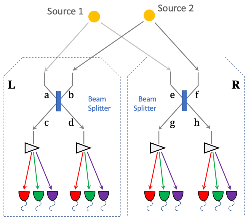
Assume there are two sources which can be observed simultaneously from two stations, L and R , with single spatial mode inputs a, b and e, f. Both sources send out photons in the form of plane wave, the path length difference between the two stations yielding phase delays \(\delta_1\) and \(\delta_2\) between the photons observed at channels a, e from source 1 and b, f from source 2, respectively. If the two detected photons are close enough in frequency and arrival time, then the pattern of coincidences measured at the outputs c, d and g, h will be sensitive to the difference in phase delays after interference at the symmetric beam splitter in each station.
\[ \Delta\delta = \delta_{1} - \delta_{2} = \frac{2\pi}{\lambda} \vec{B} \cdot (\hat{s_1} - \hat{s_2}) + \psi \]
where \(\vec{B}\) is the baseline of the two detectors and ψ is a constant phase-shift due to instrumental path length difference between the two telescope. And here Δδ encodes the relative separation between the two sources.
Procedure of Bayesian Analysis.
The analysis involves two parts:
- Simulate coincidences following Poisson process
- Feed the sampled data to MCMC and see if we can recover the original parameters used such as visibility and the separation between two sources.
Simulating Coincidence
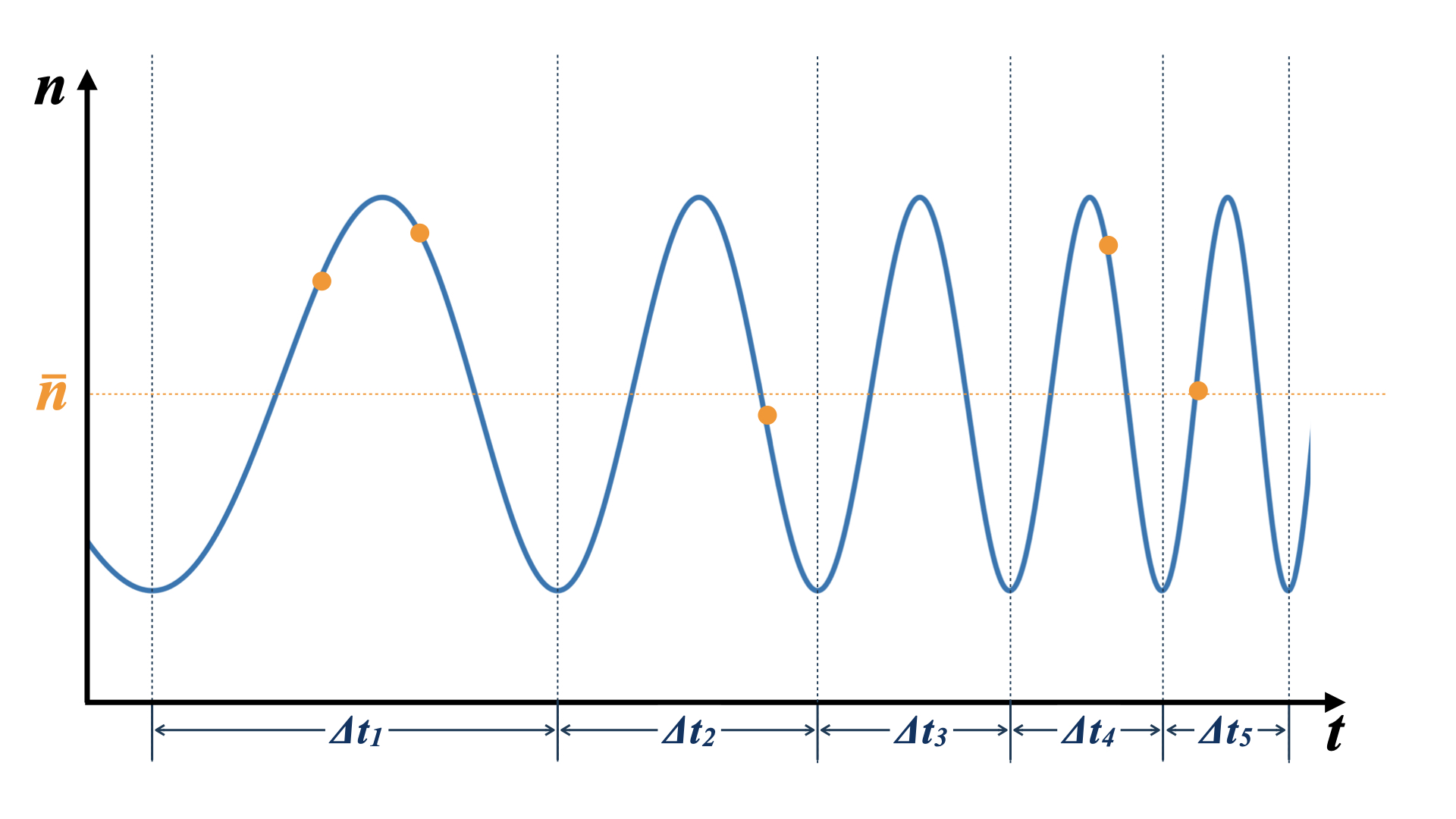
Figure 1: Schematic picture the fringe pattern. The blue curve represents a theoretical fringe pattern, and orange points are events detected.
Summary:
- Since fringes will vary in frequency as Earth rotates, we first determine the period of each fringe cycle denoted by Δt’s.
- Determine the number of detections within each fringe cycle via \(\bar{n} \times \Delta t\)
- Determine the phase, φ, of these events in each fringe cycle.
- Find the timestamp of these events corresponding to the phase, φ.
We knew the rate for different two-photon coincidence rate type (i.e. the blue curve) will be in the form:
\[ R_{\pm}(t) = \bar{n} \left(1 \pm V \cos(\delta_1 - \delta_2) \right) \]
where \(\bar{n}\) is the fringed-average value of R, and V is the fringe visibility calculated from the fluxes of the two sources. We can determine Δt’s from the curve, as well as the number of events in each fringe cycle.
Now the form of R(t) tells us that the probability density function is of the form:
\[ PDF(x) = \frac{1 \pm V\cos{(x)}}{2\pi} \quad \quad \quad x\in[-\pi, \pi] \]
and the cumulative density function (CDF) after integrating PDF from -π to φ.
\[ CDF(\phi) = \frac{\phi \pm V\sin{(\phi)} + \pi}{2\pi} \quad \quad \quad \phi\in[-\pi, \pi] \]
With a random number generator following Poisson distribution, we feed a number from 0 to 1 to CDF. By inverting the CDF, we then obtain the phase, φ, representing a coincidence. After obtaining φ for each fringe cycle, we can just find the corresponding timestamp corresponding to R(t).
MCMC Sampling
After simulating our data points following Poisson distribution, now we explore the posterior using MCMC procedure. There are 4 parameters to vary, visibility, V, separation of the two sources in the east-west direction Δd_E, north-south direction Δd_N, and the arbitrary phase, ψ.
The result gives a bunch of triangle correlation plots showing correlation between different parameters.
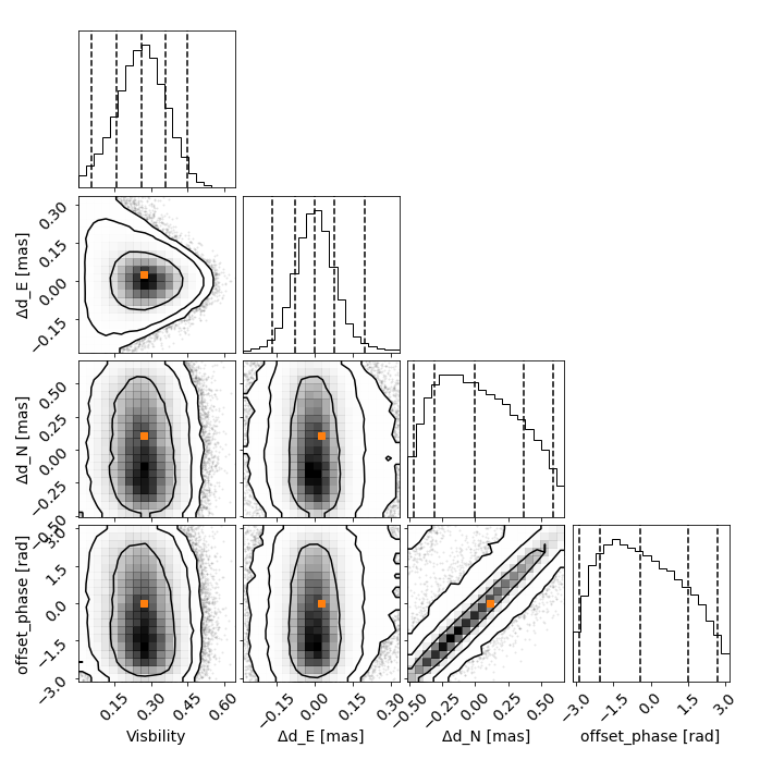
Figure 2: Triangle correlation polots generated via the corner package. The vertical dashed lines represent 2.3%, 16%, 50%, 84%, and 99.4% quantiles of the GAussian. The orange point indicate the true value of each parameter.
Result
In the end, I was able to show two telescopes with an effective collecting area of \(\sim 2\text{m}^2\), we could detect fringing and measure the astrometric separation of the sources at \(\sim\) 100 µas of precision in a few hours of observations.
This work is published in Physical Review D